Last month’s tip discussed the new Top-50 Table Viewer, one of the new additions to CALPUFF View Version 10.0 which aids modelers in visualizing output from the CALPOST postprocessor. Another addition to this release of CALPUFF View is the Ranked Values Grid View.
CALPOST’s Ranked Values are similar to the “Highest Values” option found in the Output Pathway of the AERMOD air dispersion model. Modelers define the ranked output value, and the model results are ordered on a receptor-by-receptor basis with the user-defined values reported.
For example, specifying a Ranked Value of 2 will return the 2nd highest value from each receptor for the selected species, process, and averaging period. CALPOST can calculate up to four ranked values ranging from the 1st to the 10th rank. After a successful CALPOST run, CALPUFF View uses the data to generate contour plots of each selected rank, species, process, and averaging period.
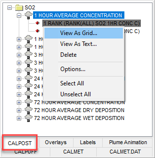
With the release of Version 10.0, modelers can now view the Ranked Values output in a gridded table viewer to extract and analyze model output more easily. To access the Ranked Values Grid View:
- Go to the CALPOST Tree View tab found in the bottom-left of the application window.
- Select the desired Ranked Values plot file from the list of species.
- Right-click the file to open the context menu.
- Select the “View As Grid” selection from this context menu.
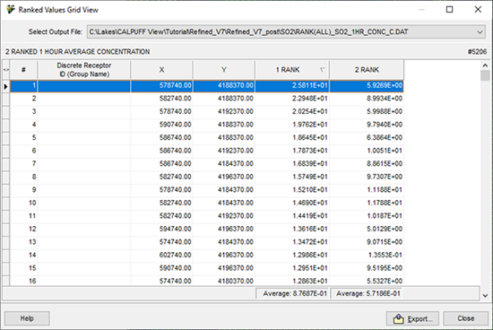
The information from the plot file is displayed in an easy-to-read grid format. The information can be sorted by column by clicking on the column header. You can also drag and drop the columns to change the order in which they are displayed. The average value of each rank column is displayed on the bottom panel, under the RANK column.
The numeric value in each RANK column represents the Ranked Value as specified in the CALPOST Options – Ranked Values settings. For example, “1 RANK” represents the highest output values (Rank 1).
At the top of this dialog, the name and location of the plot file is displayed. From this drop-down list you can select which plot file you wish to view in grid format. Below this, a description of the plot file can be seen along with the total number of receptors.
The data can also be exported to CSV format using the export button at the bottom of the dialog.